Probability

Probability is the branch of mathematics that studies the likelihood of events happening. Fundamentally, probability is about predicting the chance of specific outcomes, quantifying uncertainty in a way that provides valuable insight across various domains. Whether flipping a coin, predicting the weather, or calculating the risk of investment, probability helps make sense of potential outcomes by assigning them values between 0 (impossible) and 1 (certain). An event with a probability closer to 1 is more likely to occur, while a probability closer to 0 means it is less likely.

Watch Video

Basic Probability Rules

Understanding basic probability rules is essential in evaluating the likelihood of combined events. The Addition Rule helps us understand the probability of either of two events occurring, while the Multiplication Rule calculates the probability of both events occurring. The Complement Rule is a useful tool for determining the probability of events not happening. Together, these rules provide a solid foundation for understanding probability, allowing us to analyze situations and make predictions in a structured way. Whether we are drawing cards, rolling dice, or forecasting weather, probability rules help us navigate uncertainty in a logical and calculated manner.

The Addition Rule

The Addition Rule helps calculate the probability of either of two events occurring. There are two cases depending on whether the events are mutually exclusive or non-mutually exclusive:

Mutually Exclusive Events:

Two events are mutually exclusive if they cannot happen at the same time. For example, when drawing a single card from a deck, the event of drawing a "heart" and the event of drawing a "spade" are mutually exclusive, because a card cannot be both a heart and a spade.

For mutually exclusive events A and B, the probability of either event occurring is given by:

P(A or B) = P(A) + P(B)

Example:

If the probability of drawing a heart is 1/4 and the probability of drawing a spade is also 1/4, then the probability of drawing a heart or a spade is:

Non-Mutually Exclusive Events:

Two events are non-mutually exclusive if they can happen at the same time. For instance, in a deck of cards, the event of drawing a "red card" and the event of drawing a "face card" are non-mutually exclusive, because some red cards are also face cards.

For non-mutually exclusive events, we must subtract the probability of both events happening (since it’s counted twice otherwise):

P(A or B) = P(A) + P(B) - P(A and B)

Example:

Find the probability of drawing either a Red card or a Face card from a standard deck of 52 cards.

Probability of a Red card P (Red Card):

There are 26 red cards in a deck (13 hearts and 13 diamonds). So,

Probability of a Face card P (Face Card):

There are 12 face cards in a deck (3 in each suit: Jack, Queen, and King). So,

Probability of a card being both Red and a Face card (Red and Face):

There are 6 red face cards (3 in hearts and 3 in diamonds).

Using the Addition Rule for probability:

P(Red or Face) = P(Red) + P(Face) - P(Red and Face)

Following is a bar graph illustrating the probabilities associated with drawing a Red card, a Face card, both Red and Face, and the combined probability of drawing either Red or Face. Each bar represents a specific probability, providing a visual comparison of each outcome.

Multiplication Rule

The Multiplication Rule is used to find the probability of both events occurring. It’s important for determining the likelihood of two events happening in succession. The formula differs based on whether the events are independent or dependent:

Independent Events:

Two events are independent if the occurrence of one event does not affect the occurrence of the other. For instance, flipping a coin and rolling a die are independent events.

For independent events 𝐴 and 𝐵

P(A and B) = P(A) x P(B)

Example:

If the probability of flipping heads on a coin is 1/2 and the probability of rolling a "4" on a die is 1/6, then the probability of getting heads and rolling a "4" is:

Dependent Events:

Two events are dependent if the outcome of one affects the probability of the other. For example, drawing two cards from a deck without replacement is a dependent event because the first draw affects the second.

For dependent events, the probability of both events occurring is

P(A and B) = P(A) x P(B|A)

where P(B|A) is the probability of 𝐵 occurring given that 𝐴 has already occurred.

Example:

If the probability of drawing an ace on the first draw from a deck is 4/52 and the probability of drawing another ace on the second draw (without replacement) is 3/51, then:

The Complement Rule

The Complement Rule is useful for finding the probability that an event does not occur. If A is an event, then the probability of A not happening, denoted P(A′), is given by:

For independent events 𝐴 and 𝐵

P(A')=1-P(A))

Example:

If the probability of raining tomorrow is 0.3, then the probability that it will not rain is:

P(No Rain)=1-0.3=0.7

The Complement Rule is helpful because sometimes it’s easier to calculate the probability of an event not occurring and then use it to find the probability of the event itself.

Formula for Probability

The fundamental probability formula is:


where:

          • P(A): The outcome we are interested in.

          • Favorable Outcomes: The number of ways the event can happen.

          • Total Outcomes: The total number of possible outcomes in the sample space.

Applications of Probability

Probability plays a crucial role in various fields by helping predict outcomes, manage risks, and analyze uncertain situations. From finance to medicine and artificial intelligence, probability enables better decision-making in complex environments.

1. Finance & Risk Management

• Used in stock market analysis to predict price movements.
• Helps assess insurance risks and premium calculations.
• Applied in credit scoring and loan approval processes.

2. Medicine & Healthcare

• Used in medical diagnosis to determine disease probabilities.
• Essential for clinical trials and drug testing.
• Helps in epidemiology to study disease spread patterns.

3. Artificial Intelligence & Machine Learning

• Forms the basis of Bayesian networks for decision-making.
• Used in predictive modeling and recommendation systems.
• Helps train AI models using probabilistic algorithms.

4. Business & Marketing

• Applied in customer behavior analysis for targeted advertising.
• Used to optimize pricing strategies based on demand probabilities.
• Helps in sales forecasting and inventory management.

5. Gaming & Sports

• Determines winning probabilities in games of chance.
• Used in sports analytics to predict match outcomes.
• Helps design fair and balanced game mechanics.

6. Engineering & Quality Control

• Used in reliability testing of machines and products.
• Helps minimize defects in manufacturing processes.
• Applied in fault detection and safety assessments.

Real Life Application Examples

1. Medication Side Effects Risk Assessment

A pharmaceutical company has developed a new medication and is conducting clinical trials to assess its safety. During the trial, participants are monitored for any side effects, particularly nausea, a common issue with similar medications.

From the data gathered:

• There’s a 10% chance that any given participant will experience mild nausea from the medication.

• There’s a 3% chance that a participant will experience severe nausea.

• Additionally, there is a 1% chance that a participant may experience both mild and severe nausea symptoms.

Based on these probabilities:

1. What is the probability that a participant will experience nausea (either mild, severe, or both) while taking the medication?

2. What is the probability that a participant will experience only mild nausea but not severe nausea?

3. What is the probability that a participant will experience no nausea symptoms at all?

Solution

Step 1: Define Events and Probabilities

• P(Mild)=0.10 : the probability of experiencing mild nausea.

• P(Severe)=0.03 : the probability of experiencing severe nausea.

• P(Both)=0.01 : the probability of experiencing both mild and severe nausea.

Step 2: Calculate Probabilities

1. Probability of experiencing nausea (either mild, severe, or both):

Using the formula for the union of two events:

So, there is a 12% probability that a participant will experience some form of nausea.

2. Probability of experiencing only mild nausea (not severe):

To find this, we subtract the probability of experiencing both mild and severe nausea from the probability of mild nausea alone:

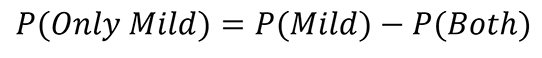
So, there is a 9% probability that a participant will experience only mild nausea.

3. Probability of experiencing no nausea symptoms at all:

To find the probability of no nausea, we calculate the complement of the probability of experiencing nausea:

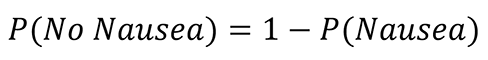
So, there is an 88% probability that a participant will experience no nausea symptoms.

Following is the probability diagram illustrating the likelihood of experiencing nausea (mild, severe, or both) from the medication. Each branch shows the probability paths based on the provided data, helping to visualize the chances of each type of nausea outcome.

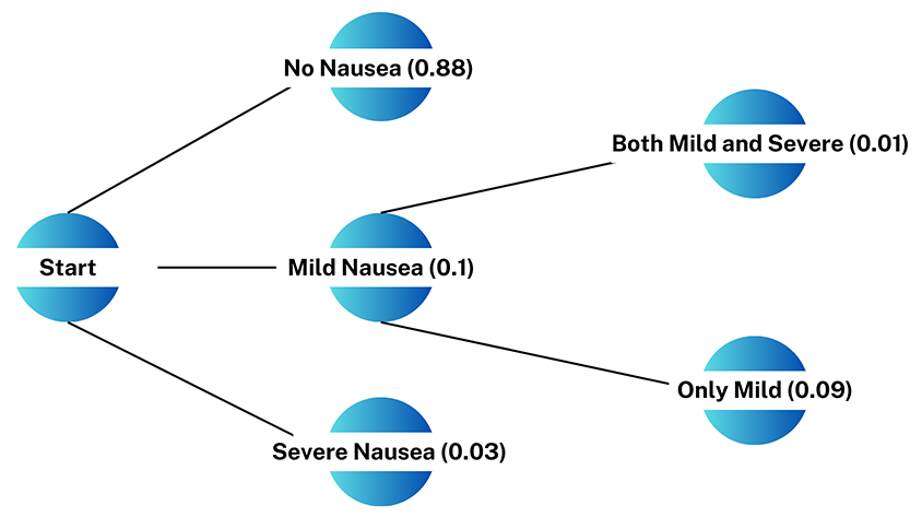
Understanding the Probability Sum

No Nausea = 0.88 (Probability of experiencing no nausea at all)

Mild Nausea = 0.10 (Probability of experiencing mild nausea, which includes "only mild" and "both mild and severe")

Severe Nausea = 0.03 (Probability of experiencing severe nausea, which already includes the cases where nausea is severe—whether alone or with mild nausea)

Thus, adding No Nausea (0.88), Mild Nausea (0.10), and Severe Nausea (0.03) gives:

0.88 + 0.10 + 0.03 = 1.01

which exceeds 1, violating the basic probability rule that the total probability of all possible outcomes must sum to exactly 1.

Where is the Overcounting?

The issue arises because "Mild Nausea (0.10)" already includes the probability of "Both Mild and Severe (0.01)", and "Severe Nausea (0.03)" also includes this same probability (0.01).

By adding 0.10 and 0.03 separately, we are counting the 0.01 probability twice. To correct for this:

P(No Nausea) + P(Mild) + P(Severe) − P (Both ) = 0.88 + 0.10 + 0.03 − 0.01 = 1.00

This correction ensures the total probability sums to 1, as required.

Final Explanation

No Nausea = 0.88 → No symptoms at all.

Mild Nausea = 0.10 → Includes both only mild nausea (0.09) and both mild and severe (0.01).

Severe Nausea = 0.03 → Includes both only severe nausea (0.02) and both mild and severe (0.01).

• Since "both mild and severe (0.01)" is counted twice when adding mild and severe separately, we must subtract it once to avoid double-counting.

Thus, the correct sum is:

0.88 + 0.10 + 0.03 - 0.01 = 1.00

This correction ensures that the total probability remains valid.


2. Political Strategy Analysis

In a certain region, a political strategist is studying voter preferences. Based on surveys:

• 60% of voters prefer Candidate A.

• 40% prefer Candidate B.

• There is also a 15% chance that a voter who prefers Candidate A may change to Candidate B based on new policy information.

What is the probability that a randomly selected voter will either prefer Candidate B initially or change to Candidate B after initially preferring Candidate A?

Solution

• P(A)=0.6 : : Probability of preferring Candidate A.

• P(B)=0.4 : Probability of preferring Candidate B.

• P(A → B)=0.15 : Probability of changing preference from A to B.

• The probability that a voter either initially prefers Candidate B or changes to Candidate B is:

P(B or A → B) = P(B) + P(A) x P(A → B)

P(B or A → B) = 0.4 + (0.6 x 0.15)

P(B or A → B) = 0.4 + 0.09 = 0.49

So, there is a 49% probability that a randomly selected voter will ultimately prefer Candidate B.

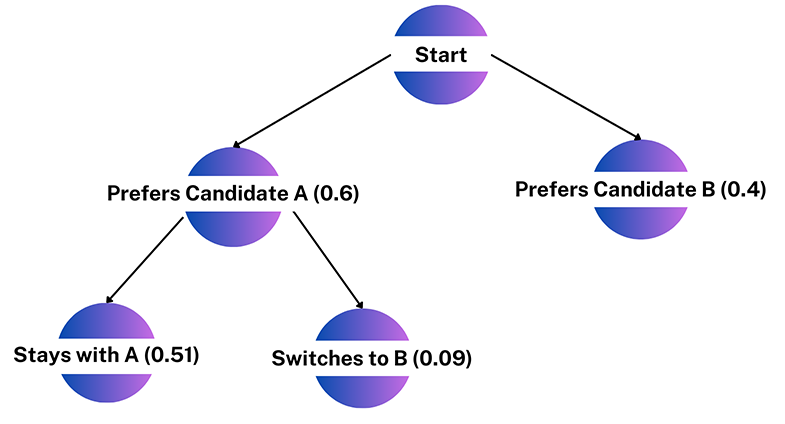
Here's the probability diagram illustrating voter preference. The diagram shows the initial preferences and the probability paths for voters either staying with or switching to Candidate B.


3. Coffee Shop

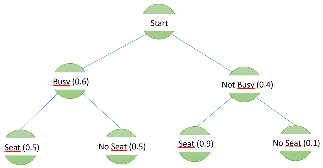
Efe is planning to visit a coffee shop every morning this week (Monday to Sunday) before work. According to past experience, he know:

• There's a 60% chance that the coffee shop will be busy when he arrives.

• When the coffee shop is busy, there's a 50% chance that he will still manage to get a seat within 5 minutes.

• If the coffee shop is not busy, there's a 90% chance he will get a seat within 5 minutes.

What is the probability that he will get a seat within 5 minutes on any given morning?

Solution

Step 1: Define Events

Let's define the events to set up the probability space:

• Let B be the event that the coffee shop is busy.

• Let S be the event that he gets a seat within 5 minutes.

P(B) = 0.6: Probability that the shop is busy.

P(B´) = 1 - P(B) = 0.4: Probability that the shop is not busy.

P(S|B) = 0.5: Probability of getting a seat within 5 minutes given that the shop is busy.

P(S|B´) = 0.9: Probability of getting a seat within 5 minutes given that the shop is not busy.

Step 2: Apply the Law of Total Probability

The probability of getting a seat within 5 minutes, P(S), is calculated using the law of total probability. This law tells us to consider all possible scenarios (in this case, the shop being busy or not)

P(S) = P(S|B) x P(B) + P(S|B´) x P(B´)

Step 3: Plug in the Values and Calculate

Substitute the given probabilities:

P(S) = (0.5 x 0.6) + (0.9 x 0.4)

P(S) = 0.3 + 0.36 = 0.66

So, the probability that you will get a seat within 5 minutes on any given morning is 0.66, or 66%.

Here’s a probability tree diagram illustrating the likelihood of each scenario. The tree shows the two main branches: the coffee shop being busy or not, followed by the probabilities of getting a seat or not within 5 minutes for each case. This visual aids in understanding how the overall probability of getting a seat is calculated by combining these pathways.

Probability Power: Understanding Uncertainty & Likelihood

Probability: Predicting Outcomes in Uncertainty

Probability helps us analyze uncertainty, predict outcomes, and make smarter decisions. Mastering probability unlocks new ways to interpret data, assess risks, and solve real-world problems with confidence!